Topic Modeling using R
Topic Modeling in R
Topic modeling provides an algorithmic solution to managing, organizing and annotating large archival text. The annotations aid you in tasks of information retrieval, classification and corpus exploration
Topic models provide a simple way to analyze large volumes of unlabeled text. A “topic” consists of a cluster of words that frequently occur together. Using contextual clues, topic models can connect words with similar meanings and distinguish between uses of words with multiple meanings. For a general introduction to topic modeling, see Probabilistic Topic Models by Steyvers and Griffiths (2007) or Introduction to Probabilistic Topic Models by David Blei (2012).
In machine learning and natural language processing topic models are generative models which provide a probabilistic framework for the term frequency occurrences in documents in a given corpus. In this example, we will be performing latent dirichlet allocation (LDA) the simplest topic model. LDA is a statistical model of document collections that tries to capture the intuition behind LDA, documents exhibit multiple topics. Blei (2102) states in his paper:
LDA and other topic models are part of the larger field of probabilistic modeling. In generative probabilistic modeling, we treat our data as arising from a generative process that includes hidden variables. This generative process defines a joint probability distribution over both the observed and hidden random variables. We perform data analysis by using that joint distribution to compute the conditional distribution of the hidden variables given the observed variables. This conditional distribution is also called the posterior distribution.
Data Processing
For this example I am using the publicly available Lessons Learned from the NASA Engineering Network. I exported the spreadsheet from the Lesson Learned database and imported it as a csv file to an R data frame. I had to do some cleaning of the data, this is the structure of the dataframe when I was done.
str(llis.display)
## 'data.frame': 1637 obs. of 11 variables:
## $ LessonId : int 9501 8018 8701 8017 8601 8016 8501 8403 8402 8401 ...
## $ Submitter1 : Factor w/ 398 levels "Abbey, George ",..: 19 19 267 19 267 360 267 267 267 195 ...
## $ Title : chr "Manhole Arc-Flash Risk Reduction" "CRCA Sampling Process Lessons Learned" "Take Special Care to Avoid Misprobing When Using Breakout Boxes" "Using Heritage Equipment From Uncontrolled Sources - Incompatible Boss Seal" ...
## $ Abstract : chr " Power system distribution at Kennedy Space Center (KSC) consists primarily of high-voltage, underground cables. These cables "| __truncated__ " The sampling and analysis processes, used to verify cleanliness of gases and liquids loaded into payloads and related Ground "| __truncated__ " An operator error involving mis-probing during a safe-to-mate procedure, in which a breakout box (BOB) was used, resulted in "| __truncated__ " The Restore Project obtained excessed equipment from the Space Shuttle Program and used this heritage equipment in a test set"| __truncated__ ...
## $ Lesson : chr " Laboratory testing revealed higher than anticipated safety risks from a potential arc-flash event in a manhole environment wh"| __truncated__ " The particle contamination monitoring was insufficient to provide meaningful feedback to ensure operating protocols were succ"| __truncated__ " The common use of BOBs during subsystem/system integration and test does much to facilitate hardware checkout and test proced"| __truncated__ " Implement a \xd2trust but verify\xd3 philosophy when using components and assemblies obtained from uncontrolled sources such "| __truncated__ ...
## $ Organization : Factor w/ 14 levels "AFRC","ARC","GRC",..: 9 9 7 9 7 9 7 7 7 7 ...
## $ LessonDate : POSIXct, format: "2014-06-06" "2014-03-11" ...
## $ MissionDirectorate: Factor w/ 20 levels "","Aeronautics Research, ",..: 6 14 6 14 5 14 15 5 15 16 ...
## $ SafetyIssue : Factor w/ 2 levels "false","true": 2 1 2 1 1 1 2 1 1 1 ...
## $ Categories : Factor w/ 376 levels "","Accident Investigation, Air-Traffic Management, Aircraft, Communication Systems, Extra-Vehicular Activity, Facilities, Flight O"| __truncated__,..: 120 1 270 238 308 303 239 177 182 266 ...
## $ DocNum : int 1 2 3 4 5 6 7 8 9 10 ...
Create the Corpus and Document Term Matrix
The first thing we need to do is import the csv file into a corpus using the tm package. The corpus will be used to construct the document term matrix for use in developing the topic model. Since I am importing a spreadsheet, I need to create a mapping for the corpus to use. The first item is the content used in the modeling, the remaining items are added as metadata to the corpus object.
m <- list(content = "Lesson", id = "LessonId", heading = "Title", authors = "Submitter1", topic = "Categories",
abstract = "Abstract", org = "Organization", data = "LessonDate", dir = "MissionDirectorate",
safetyissue = "SafetyIssue", docnum = "DocNum", topic = "Topic")
The Corpus function in the tm package returns a Corpus object holding all of the lessons and metadata. This will take up some memory, so plan accordingly. In this case the corpus object was 235.3 MB while the csv was less than 2 MB.
llis.corpus <- tm::Corpus(tm::DataframeSource(llis.display), readerControl = list(reader = tm::readTabular(mapping = m)))
Using the corpus we create the document term matrix, a mathematical matrix that describes the frequency of terms that occur in a collection of documents. In a document-term matrix, rows correspond to documents in the collection and columns correspond to terms.
llistopic.dtm <- tm::DocumentTermMatrix(llis.corpus, control = list(stemming = TRUE, stopwords = TRUE,
minWordLength = 2, removeNumbers = TRUE, removePunctuation = TRUE))
At this point I have all of the terms in the corpus with the exception of common stopwords. The terms have been stemmed, punctuation and numbers have been removed and I only kept words that had at minimum two characters. That left me with 59049 terms.
str(llistopic.dtm)
## List of 6
## $ i : int [1:59049] 1 1 1 1 1 1 1 1 1 1 ...
## $ j : int [1:59049] 23 369 411 425 453 827 996 1394 1406 1463 ...
## $ v : num [1:59049] 1 1 1 2 2 1 1 2 1 1 ...
## $ nrow : int 1637
## $ ncol : int 8427
## $ dimnames:List of 2
## ..$ Docs : chr [1:1637] "9501" "8018" "8701" "8017" ...
## ..$ Terms: chr [1:8427] "aatt" "abandon" "abate" "abbrevi" ...
## - attr(*, "class")= chr [1:2] "DocumentTermMatrix" "simple_triplet_matrix"
## - attr(*, "weighting")= chr [1:2] "term frequency" "tf"
A common way to reduce the number of terms is to use the term frequency inverse document frequecy (tf-idf), a numerical statistic that is intended to reflect how important a word is to a document in a collection or corpus. The tf-idf value increases proportionally to the number of times a word appears in the document, but is offset by the frequency of the word in the corpus, which helps to adjust for the fact that some words appear more frequently in general. I will use it as a weighting factor to trim the number of terms I will use in the model.
term_tfidf <- tapply(llistopic.dtm$v/slam::row_sums(llistopic.dtm)[llistopic.dtm$i], llistopic.dtm$j, mean) *
log2(tm::nDocs(llistopic.dtm)/slam::col_sums(llistopic.dtm > 0))
summary(term_tfidf)
## Min. 1st Qu. Median Mean 3rd Qu. Max.
## 0.003813 0.089720 0.155000 0.217300 0.266900 3.559000
The summary for the tf-idf shows a median of 0.155. This will used as my lower limit, removing terms from the document term matrix with a tf-idf smaller than 0.155, ensuring very frequent terms are omitted. The new median is 2.
## Keeping the rows with tfidf >= to the 0.155
llisreduced.dtm <- llistopic.dtm[,term_tfidf >= 0.155]
summary(slam::col_sums(llisreduced.dtm))
## Min. 1st Qu. Median Mean 3rd Qu. Max.
## 1.000 1.000 2.000 6.056 6.000 196.000
Determine k number of topics
A lot of the following work is based on Martin Ponweiser’s thesis, Latent Dirichlet Allocation in R. One aspect of LDA, is you need to know the k number of optimal topics for the documents. From Martins work, I am using a harmonic mean method to determine k, as shown in section 4.3.3, Selection by Harmonic Mean.
The harmonic mean function:
harmonicMean <- function(logLikelihoods, precision = 2000L) {
llMed <- median(logLikelihoods)
as.double(llMed - log(mean(exp(-mpfr(logLikelihoods,
prec = precision) + llMed))))
}
First, an example of finding the harmonic mean for one value of k, using a burn in of 1000 and iterating 1000 times. `Keep’ indicates that every keep iteration the log-likelihood is evaluated and stored. The log-likelihood values are then determined by first fitting the model. This returns all log-likelihood values including burn-in, i.e., these need to be omitted before calculating the harmonic mean:
k <- 25
burnin <- 1000
iter <- 1000
keep <- 50
fitted <- topicmodels::LDA(llisreduced.dtm, k = k, method = "Gibbs",control = list(burnin = burnin, iter = iter, keep = keep) )
## assuming that burnin is a multiple of keep
logLiks <- fitted@logLiks[-c(1:(burnin/keep))]
## This returns the harmomnic mean for k = 25 topics.
harmonicMean(logLiks)
## [1] -162256.9
To find the best value for k for our corpus, we do this over a sequence of topic models with different vales for k. This will generate numerous topic models with different numbers of topics, creating a vector to hold the k values. We will use a sequence of numbers from 2 to 100, stepped by one. Using the lapply function, we run the LDA function using all the values of k. To see how much time is needed to run the process on your system, use the system.time function. I ran this on a 2.9 GHz MAC, running 10.10.3 with 32 GB of ram.
seqk <- seq(2, 100, 1)
burnin <- 1000
iter <- 1000
keep <- 50
system.time(fitted_many <- lapply(seqk, function(k) topicmodels::LDA(llisreduced.dtm, k = k,
method = "Gibbs",control = list(burnin = burnin,
iter = iter, keep = keep) )))
## user system elapsed
## 3748.759 4.641 3764.411
# extract logliks from each topic
logLiks_many <- lapply(fitted_many, function(L) L@logLiks[-c(1:(burnin/keep))])
# compute harmonic means
hm_many <- sapply(logLiks_many, function(h) harmonicMean(h))
Now that is have calculated the harmonic means of the models for 2 - 100 topics, you can plot the results using ggplot2 package.
ldaplot <- ggplot(data.frame(seqk, hm_many), aes(x=seqk, y=hm_many)) + geom_path(lwd=1.5) +
theme(text = element_text(family= NULL),
axis.title.y=element_text(vjust=1, size=16),
axis.title.x=element_text(vjust=-.5, size=16),
axis.text=element_text(size=16),
plot.title=element_text(size=20)) +
xlab('Number of Topics') +
ylab('Harmonic Mean') +
annotate("text", x = 25, y = -80000, label = paste("The optimal number of topics is", seqk[which.max(hm_many)])) +
ggtitle(expression(atop("Latent Dirichlet Allocation Analysis of NEN LLIS", atop(italic("How many distinct topics in the abstracts?"), ""))))
ldaplot
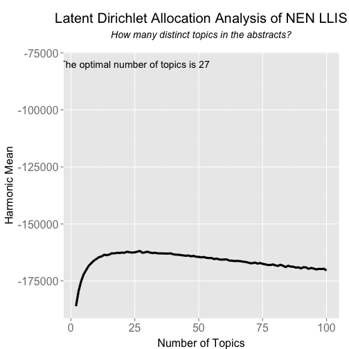
If you just want to know the optimal number of topics:
seqk[which.max(hm_many)]
## [1] 27
Time to run the Model
To run the model, I am using the LDA function in the topicmodels package. You pass the document term matrix, optimal number of topics, the estimation method, how many iterations to do and a seed number if you want to be able to replicate the results.
system.time(llis.model <- topicmodels::LDA(llisreduced.dtm, 27, method = "Gibbs", control = list(iter=2000, seed = 0622)))
## user system elapsed
## 19.662 0.023 19.721
Explore the model
The topics function from the package is used to extract the most likely topic for each document and the terms function to extract the terms per topic. The terms are listed in rank order, with the most frequent term in the topic listed first. The most diagnostic topic for each document is added to the llis data frame. This will be used in the visualization component of this analysis, Graphing a Lesson Learned Database for NASA Using Neo4j, R/RStudio & Linkurious.
llis.topics <- topicmodels::topics(llis.model, 1)
## In this case I am returning the top 30 terms.
llis.terms <- as.data.frame(topicmodels::terms(llis.model, 30), stringsAsFactors = FALSE)
llis.terms[1:5]
## Topic 1 Topic 2 Topic 3 Topic 4 Topic 5
## 1 electron report softwar reliabl power
## 2 tool gse simul loss crane
## 3 user code instrument comput voltag
## 4 nesc document vent redund output
## 5 pyro mishap blanket class suscept
## 6 home incid back aircraft suppli
## 7 peer logist endtoend fuel switch
## 8 travel main terra care subsystem
## 9 consequ investig brspan proven laboratori
## 10 transient polici sts catastroph certifi
## 11 box worker commerci parts light
## 12 larc secur caviti termin relay
## 13 protect deck link inflight clean
## 14 power attend maneuv vehicle extrem
## 15 pyrotechn electr array long metadyn
## 16 startup pressur mco parameters draw
## 17 instrument supervisor code secur upgrad
## 18 injuri unsaf fidel find accord
## 19 particl wit frcs wait hybrid
## 20 simpl facil fsw calcul segment
## 21 subsystem anomali routin envelop constraint
## 22 financi manhol trajectori accur deterior
## 23 problems slow brimg reliability lifecycl
## 24 arm uniform bulkhead term malfunct
## 25 assumpt adeosii frc card reentri
## 26 email hazard pvd fabric structure
## 27 interact intern resources flux infrastructur
## 28 logic constitut target meteoroid loop
## 29 other dissent upgrad research shown
## 30 supervisor email workaround structur spare
# Creates a dataframe to store the Lesson Number and the most likely topic
doctopics.df <- as.data.frame(llis.topics)
doctopics.df <- dplyr::transmute(doctopics.df, LessonId = rownames(doctopics.df), Topic = llis.topics)
doctopics.df$LessonId <- as.integer(doctopics.df$LessonId)
## Adds topic number to original dataframe of lessons
llis.display <- dplyr::inner_join(llis.display, doctopics.df, by = "LessonId")
As part of the visualization I will construct later, a topic label needs be used to created. The terms are gathered in rank order and then the label is created by concatenating the first three terms.
topicTerms <- tidyr::gather(llis.terms, Topic)
topicTerms <- cbind(topicTerms, Rank = rep(1:30))
topTerms <- dplyr::filter(topicTerms, Rank < 4)
topTerms <- dplyr::mutate(topTerms, Topic = stringr::word(Topic, 2))
topTerms$Topic <- as.numeric(topTerms$Topic)
topicLabel <- data.frame()
for (i in 1:27){
z <- dplyr::filter(topTerms, Topic == i)
l <- as.data.frame(paste(z[1,2], z[2,2], z[3,2], sep = " " ), stringsAsFactors = FALSE)
topicLabel <- rbind(topicLabel, l)
}
colnames(topicLabel) <- c("Label")
topicLabel
## Label
## 1 electron tool user
## 2 report gse code
## 3 softwar simul instrument
## 4 reliabl loss comput
## 5 power crane voltag
## 6 wire electr check
## 7 build sourc batteri
## 8 crew iss equipment
## 9 shuttl leak seal
## 10 mainten ksc repair
## 11 document human osp
## 12 procedur iampt lesson
## 13 vendor technolog cot
## 14 investig board circuit
## 15 damag fire hazard
## 16 excess posit move
## 17 materi transfer properti
## 18 thermal element temperatur
## 19 loss command fault
## 20 cabl optic motor
## 21 jpl scienc missions
## 22 contamin surfac clean
## 23 fund structur bull
## 24 nbsp joint defect
## 25 pressur valv propel
## 26 research protect effici
## 27 abort performance subsystem
Working With Theta
One of the posterior items generated by the model is the per document probabilities of the topics. You extract theta using the posterior function from the topicmodels package. The result displayed is the theta for Topic 1 -5 of the first 6 documents.
theta <- as.data.frame(topicmodels::posterior(llis.model)$topics)
head(theta[1:5])
## 1 2 3 4 5
## 9501 0.01949318 0.03001949 0.03001949 0.01949318 0.01949318
## 8018 0.04916986 0.03192848 0.04916986 0.03192848 0.03192848
## 8701 0.03192848 0.03192848 0.03192848 0.03192848 0.04916986
## 8017 0.02986858 0.02986858 0.02986858 0.02986858 0.04599761
## 8601 0.02153316 0.04478898 0.02153316 0.02153316 0.03316107
## 8016 0.03248863 0.03248863 0.03248863 0.03248863 0.05003249
We can correlate the topic by the metadata available, here will will use the predefined category of the documents. I construct a dataframe binding the Document Number, theta for the document, and its associated category. The column means of theta, grouped by category is calculated.
x <- as.data.frame(row.names(theta), stringsAsFactors = FALSE)
colnames(x) <- c("LessonId")
x$LessonId <- as.numeric(x$LessonId)
theta2 <- cbind(x, theta)
theta2 <- dplyr::left_join(theta2, FirstCategorybyLesson, by = "LessonId")
## Returns column means grouped by catergory
theta.mean.by <- by(theta2[, 2:28], theta2$Category, colMeans)
theta.mean <- do.call("rbind", theta.mean.by)
I can now correlate the topics.
library(corrplot)
c <- cor(theta.mean)
corrplot(c, method = "circle")
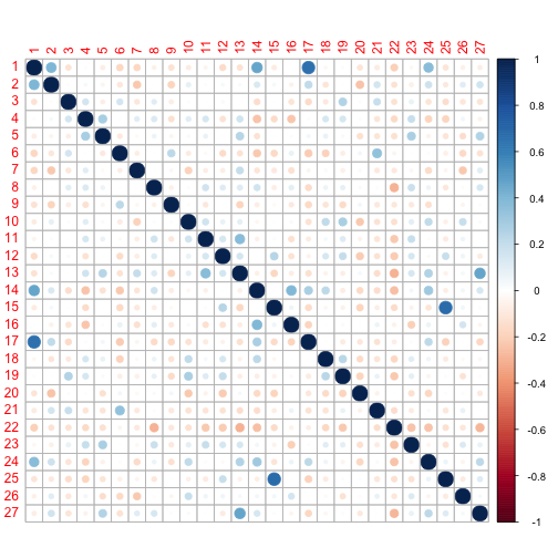
Using the categories mean theta, it is possible to select the most diagnostic topic for each of the categories.
theta.mean.ratios <- theta.mean
for (ii in 1:nrow(theta.mean)) {
for (jj in 1:ncol(theta.mean)) {
theta.mean.ratios[ii,jj] <-
theta.mean[ii,jj] / sum(theta.mean[ii,-jj])
}
}
topics.by.ratio <- apply(theta.mean.ratios, 1, function(x) sort(x, decreasing = TRUE, index.return = TRUE)$ix)
# The most diagnostic topics per category are found in the theta 1st row of the index matrix:
topics.most.diagnostic <- topics.by.ratio[1,]
head(topics.most.diagnostic)
## Accident Investigation
## 3
## Acquisition / procurement strategy and planning
## 23
## Administration / Organization
## 27
## Aerospace Safety Advisory Panel
## 22
## Aircraft
## 9
## Categories
## 16
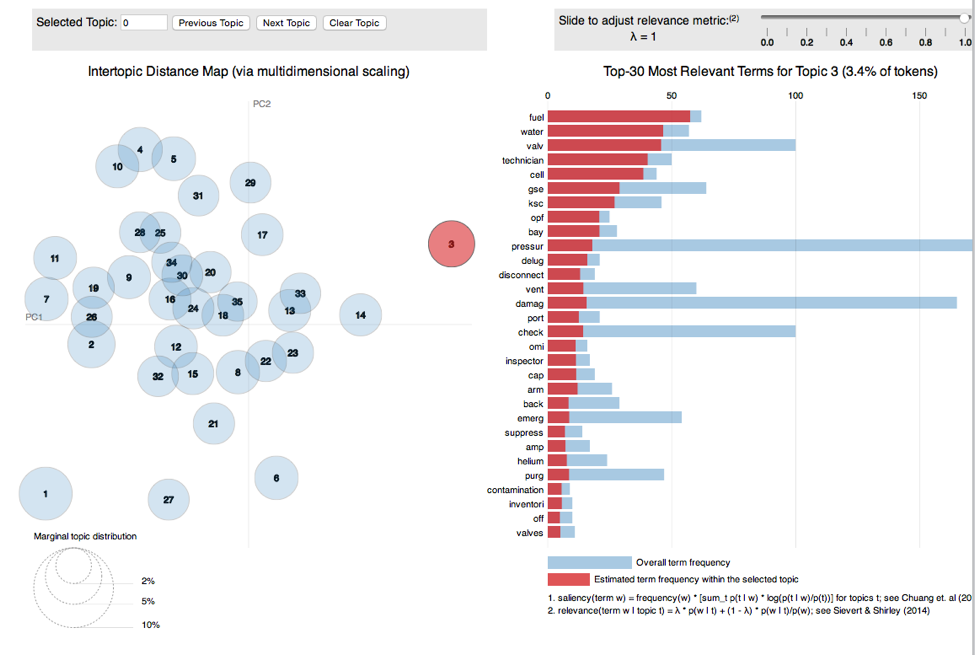
Visualizing the Model In R
The LDAvis package provides an excellent way to visualize the topics and terms associated with them.
However converting your values to work with LDAvis can be daunting. I found a function at this site to make the conversion from topicmodels output to LDAvis JSON input easier. The linking function, called topicmodels_json_ldavis, is below. To use it follow these steps:
- Convert the output of a topicmodels Latent Dirichlet Allocation to JSON for use with LDAvis
- @param fitted Output from a topicmodels
LDAmodel. - @param corpus Corpus object used to create the document term matrix for the
LDAmodel.- This should have been create with the tm package’s
Corpusfunction.
- This should have been create with the tm package’s
- @param doc_term The document term matrix used in the
LDAmodel. This should have been created with the tm package’sDocumentTermMatrixfunction.
- @see also
LDAvis. - @export
- Load the function.
topicmodels_json_ldavis <- function(fitted, corpus, doc_term){
## Required packages
library(topicmodels)
library(dplyr)
library(stringi)
library(tm)
library(LDAvis)
## Find required quantities
phi <- posterior(fitted)$terms %>% as.matrix
theta <- posterior(fitted)$topics %>% as.matrix
vocab <- colnames(phi)
doc_length <- vector()
for (i in 1:length(corpus)) {
temp <- paste(corpus[[i]]$content, collapse = ' ')
doc_length <- c(doc_length, stri_count(temp, regex = '\\S+'))
}
temp_frequency <- inspect(doc_term)
freq_matrix <- data.frame(ST = colnames(temp_frequency),
Freq = colSums(temp_frequency))
rm(temp_frequency)
## Convert to json
json_lda <- LDAvis::createJSON(phi = phi, theta = theta,
vocab = vocab,
doc.length = doc_length,
term.frequency = freq_matrix$Freq)
return(json_lda)
}
The function creates a json file to pass to LDAvis, by supplying the fitted model, corpus and document term matrix used. The ‘serVis` function opens a viewer for you to explore the topics and terms. Below is an image of what the viewer would look like when opened.
llis.json <- topicmodels_json_ldavis(llis.model, llis.corpus, llisreduced.dtm)
serVis(llis.json)